Theme 3: Pollution from our activities

Our environment is polluted when substances or kinds of energy (noise, light, heat) enter it and cause harm.

Image: Ministry for the Environment
Some pollutants directly affect our health. Bacteria like Campylobacter in drinking water can cause illness, and very fine particles in the air can cause lung and heart problems. Other pollutants pose threats to the health of plants, animals, and ecosystems, like plastic waste in the ocean or excess nutrients in our waterways. Pollution also affects our connections to nature. Artificial light from towns and cities reduces our view of the night sky, and murky streams spoil our enjoyment of these environments.
Most pollution comes from human activities, such as industry, agriculture, power generation, home heating, and transport, but some comes from natural events like volcanic eruptions. Often pollution has a mix of sources. Waterways, for example, can contain disease-causing bacteria from bird faeces, nutrients from farm run-off, and heavy metals from vehicle wear (copper from brake pads and zinc from tyres).
Pinpointing the cause of pollution can be difficult. Some pollution comes from one place (eg a factory or sewage treatment plant) while other pollution has many sources (eg vehicle emissions). Pollutants can move in the air, in water, and through soil, often over large distances and long periods of time. They can also change their form, sometimes becoming more-hazardous pollutants.
This theme focuses on two kinds of pollution that are considered of most importance to New Zealand, based on the criteria listed earlier in A focus on what matters:
Other issues highlighted in this report also contribute to or are related to pollution:
Waterways in farming areas are polluted by excess nutrients, pathogens, and sediment. This threatens our freshwater ecosystems and cultural values, and may make our water unsafe for drinking and recreation.
It affects almost all rivers and many aquifers in farming areas. Some lakes and estuaries may also be affected.
In areas of pastoral farming the median concentrations of nutrients, pathogens, and sediment in rivers are between 2 and 15 times higher than natural conditions.
It is difficult to reverse because farming is important for the economy, some catchments respond slowly to interventions, the issue is widespread, and departure from natural conditions is large.
71 percent of river length in areas of pastoral farming has modelled levels of nitrogen that may cause some growth effect on aquatic species, and 82 percent of river length in farmed areas has modelled pathogen levels that pose risks to human health from swimming. Both degrade cultural well-being.
There is poor understanding and insufficient data for exactly where, when, and what farming and farm management practices have contributed to or mitigated the observed state and trends.
Understanding water quality and why it varies from location to location and over time is challenging. Part of the difficulty arises because rivers, lakes, and groundwaters are parts of an interconnected freshwater system that flows into estuaries and coastal environments. A reduction in water quality in one part of the system can affect water quality elsewhere and make it difficult to determine the sources of pollution. Polluted groundwater, for instance, can flow into a river that flows into an estuary. Also, pollution moves slowly through some catchments, so the water quality in some locations today may be the result of land use that occurred many years ago (see Lag times can be long).
Catchments can contain a mix of land-cover types and land uses, like native vegetation, exotic forest, urban areas, and farming (ie agriculture), which can affect water quality in different ways. As used in this report, farming refers to pastoral farming (including dairy, beef, sheep, and other livestock), horticulture, and arable cropping. Different types of farming can also have a variety of effects on water quality – depending on the characteristics of the farmed land and the way the farming is managed. For example, some farm management practices, like keeping stock out of streams or riparian planting, can mitigate or limit the impacts on water quality (Larned et al, 2018a), but information about the types of management practices on specific farms is not generally available.
Despite these challenges to understanding water quality, there is clear evidence that waterways in our farming areas have markedly higher pollution by nutrients (nitrogen and phosphorus), microbial pathogens, and sediment than waterways in native catchments. Although all these pollutants occur naturally in freshwater systems, excess concentrations can cause harm. (See Issue 5: Our environment is polluted in urban areas for a comparison between water quality in farming and urban environments.)
Nitrogen and phosphorus are essential nutrients for plants, and small amounts are a natural component of healthy freshwater ecosystems. Different forms of nitrogen and phosphorus have different properties:
When nitrogen and phosphorus accumulate in rivers, lakes, and enclosed coastal waters above certain concentrations (referred to as nutrient enrichment), they can stimulate excessive growth of algae, water weeds, and cyanobacteria. At very high concentrations, nitrate-nitrogen and ammonia (a form of ammoniacal nitrogen) can be toxic to aquatic life. Very high concentrations of nitrate-nitrogen also make water unsafe to drink. Little is known about the effects of nutrient enrichment on groundwater ecosystems.
Several pathogens cause disease if they are consumed by people, like Campylobacter bacteria, the protozoa Giardia and Cryptosporidium, and some types of viruses. These pathogens can cause rapid and major outbreaks of illness and limit how we use our fresh water for drinking and recreation. The possible presence of pathogens is assessed by monitoring the levels of the indicator bacteria E. coli in fresh water, or Enterococci and faecal coliforms in sea water. Finding these indicator organisms in water is a reliable sign that it contains animal or human faeces, which signals that pathogens may be present. Some pathogens, such as toxoplasmosis, can also persist for months in coastal seas.
Sediment includes all the solid particles carried by and in water. Fine particles like silt, mud, and organic material can reduce clarity (underwater visibility) and increase turbidity (cloudiness) in rivers, lakes, and coastal waters. Poor clarity and high turbidity affect the habitat and food supply of aquatic life, like fish and birds, and the growth of aquatic plants. Excess fine sediment that settles onto the bottom of rivers, lakes, and estuaries can smother aquatic ecosystems. Excess sediment can also have an impact on the aesthetic values and recreational use of rivers, lakes, and coastal areas.
This report assesses the current state of water quality against two sets of guidelines and thresholds (see Water quality guidelines and thresholds below). A comparison with the water quality under estimated natural conditions is based on the default guideline values in the latest Australian and New Zealand guidelines for fresh and marine water quality (ANZG, 2018). A comparison with water quality that may cause effects on ecosystem health or human health for recreation is based on the National Objectives Framework in the National Policy Statement for Freshwater Management 2014 (Amended 2017) (MfE, 2017b).
Note: All gross domestic product (GDP) figures are from the National accounts (Industry production and investment): year ended March 2017. These figures exclude manufacturing or processing of primary products. They are in current prices, ie not adjusted for the effect of changing prices over time. The people employed information is from linked employer-employee data (LEED). The measure is main earning source, by industry using New Zealand standard industry output categories.
This report predominantly uses two sets of guidelines and thresholds to assess the state of water quality.
The Australian and New Zealand guidelines for fresh and marine water quality (ANZG, 2018) define default guideline values (DGVs) that correspond to the concentrations of the water quality variables that are estimated to occur in natural conditions. The DGVs describe environmental conditions expected in the absence of human influence and focus on ecosystem health. DGVs are not standards that have to be met. Rather, if a DGV is exceeded it prompts further analysis and monitoring to find out if an aquatic ecosystem has enough protection.
DGVs have been defined for river water quality and sedimentation in estuaries, but not for other aspects of water quality in groundwater, lakes, or estuaries.
The National Policy Statement for Freshwater Management (Freshwater NPS) (MfE, 2017b) requires councils to set objectives for freshwater management in their regional plans. The National Objectives Framework (NOF), a part of the Freshwater NPS, helps local authorities and communities set these freshwater management objectives.
The NOF defines minimum acceptable states for water quality based on ecosystem health and human health.
The NOF defines bands (ranges) for relevant variables to support these values in rivers and lakes. The NOF bands represent different states, with A being the best state and D or E the worst. This includes setting minimum acceptable states called national bottom lines that councils must meet, or work towards meeting over time. The national bottom line is the boundary between bands C and D.
The bands are designed to help communities make decisions on how to manage water quality. For example, the NOF includes bands for the concentrations of Escherichia coli (E. coli) in relation to the risk of infection by Campylobacter during swimming in rivers and lakes, and bands for concentrations of nitrate-nitrogen and ammonia in relation to toxicity effects on aquatic species.
Councils are also required to maintain or improve water quality – they cannot allow water quality to drop from band A to band B for example.
Note that the NOF bands are not directly comparable to the DGVs in the Australian and New Zealand guidelines for fresh and marine water quality.
Many studies at national, regional, and catchment scales show that concentrations of nitrogen, phosphorus, fine sediment, and E. coli in rivers all increase as the area of farmland upstream increases (Larned et al, 2018a). This section focuses on pastoral farming, for which most data is available and which occurs over much more land area than horticulture or growing arable crops (Larned et al, 2018a).
Computer models have been developed to estimate the water quality in New Zealand rivers (figure 8 for example, shows nitrate-nitrogen concentrations). This report uses four categories – pastoral, urban, exotic forest, and native – to classify monitoring sites and stretches (or reaches) of rivers according to the type of land cover in the catchment upstream. (Note: Land-cover class is determined by the spatially dominant land-cover type in the upstream catchment, unless pasture exceeds 25 percent of catchment area, in which case the pastoral class is assigned, or unless urban cover exceeds 15 percent of catchment area, in which case the urban class is assigned. Any catchment includes a mixture of land cover, but each river reach is assigned to one of four land-cover categories for the purpose of this report.)
River pollution can be assessed (degree and spatial extent) by comparing the modelled water quality in the native land and pastoral classes. The river water quality expected for native land cover, ie in natural conditions, is shown by the DGVs in the Australian and New Zealand guidelines for fresh and marine water quality (ANZG, 2018). Comparing against expected natural conditions, although not a perfect measure, gives a benchmark to assess the scale of change against. The same approach is used in Issue 5: Our environment is polluted in urban areas, where river water quality is compared for the urban and native land-cover classes.
The models show that, for most water quality variables, 50–90 percent of the total river length in the pastoral land-cover class exceeds the relevant DGV for 2013–17 (see table 1). In comparison, the models show that DGVs are exceeded in less than 30 percent of the river length in the native land-cover class. (A total of 188,024 kilometres of New Zealand’s river length is in the pastoral land-cover class, whereas a total of 198,126 kilometres is in the native land-cover class.)

Image: NIWA (Data source)
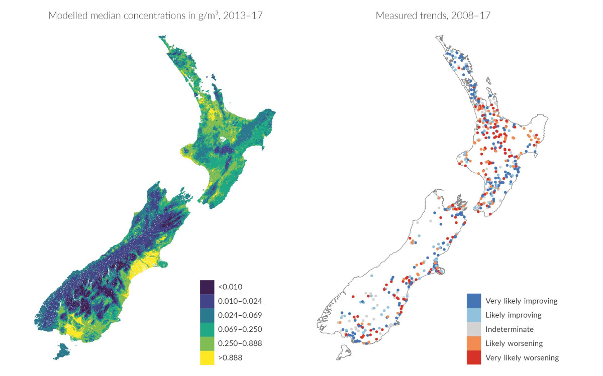
Image: NIWA (Data source)
From 2013 to 2017, compared with rivers in the native land-cover class, the pastoral land-cover class had modelled median nitrate-nitrogen levels that were 9.7 times higher, dissolved reactive phosphorus levels 3.4 times higher, turbidity 2.2 times higher, and E. coli levels 14.6 times higher (see table 1).
Lake, coastal, and estuarine water quality monitoring sites are not categorised by the amount of farmland in their catchments, so the impacts of farming cannot be specifically assessed. (See indicators: Lake water quality and Coastal and estuarine water quality.)
The quality of groundwater varies across New Zealand. Nationally over the period 2010–14, 34 percent of 342 sites had median nitrate-nitrogen concentration greater than 3 grams per cubic metre. These values indicate that groundwater in these locations has been influenced by industrialised agriculture and is highly likely to have been impacted by human activity, based on national-scale studies in New Zealand (Morgenstern & Daughney, 2012; Daughney & Reeves, 2005). Expected levels in natural conditions have not yet been defined for other groundwater quality parameters (like phosphorus or E. coli).
Groundwater quality monitoring sites are not categorised according to land use, so the specific effects of farming cannot be identified. However, some patterns coincide with pastoral land cover – especially nitrate-nitrogen in Canterbury (see figure 9 compared with figure 4). (See indicator: Groundwater quality.)
| Modelled median value of water quality variable, 2013–17 | River length (km) that does not meet ANZG DGV | ||||
|---|---|---|---|---|---|
| Water quality variable | Units | Pastoral land cover | Native land cover | Pastoral land cover | Native land cover |
| Total nitrogen | mg/m3 | 738.6 | 115.9 | 162,475 (86%) | 57,027 (29%) |
| Nitrate-nitrogen | mg/m3 | 246.6 | 25.6 | 155,000 (82%) | 26,610 (13%) |
| Ammoniacal nitrogen | mg/m3 | 8.3 | 4.0 | 94,237 (50%) | 29,464 (15%) |
| Total phosphorus | mg/m3 | 32.5 | 8.3 | 169,142 (90%) | 50,977 (26%) |
| Dissolved reactive phosphorus | mg/m3 | 14.6 | 4.4 | 144,191 (77%) | 45,270 (23%) |
| E. coli | cfu/100 ml | 195.0 | 13.3 | 47,314 (25%) | 1,117 (0.6%) |
| Turbidity | NTU | 2.9 | 1.3 | 117,343 (62%) | 22,962 (12%) |
| Clarity | m | 1.7 | 3.3 | 13,499 (7%) | 1,467 (1%) |
Note: ANZG (2018) does not include a DGV for E. coli, so the expected concentration for natural conditions is based on the guideline value determined by McDowell et al (2013). Because of the way a DGV is defined, under natural conditions it is expected that about 20 percent of river length will not meet the DGVs and about 5 percent of river length will not meet the E. coli guideline.
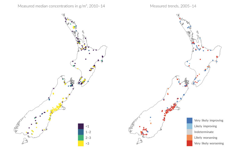
Image: Regional councils; GNS Science (Data source)
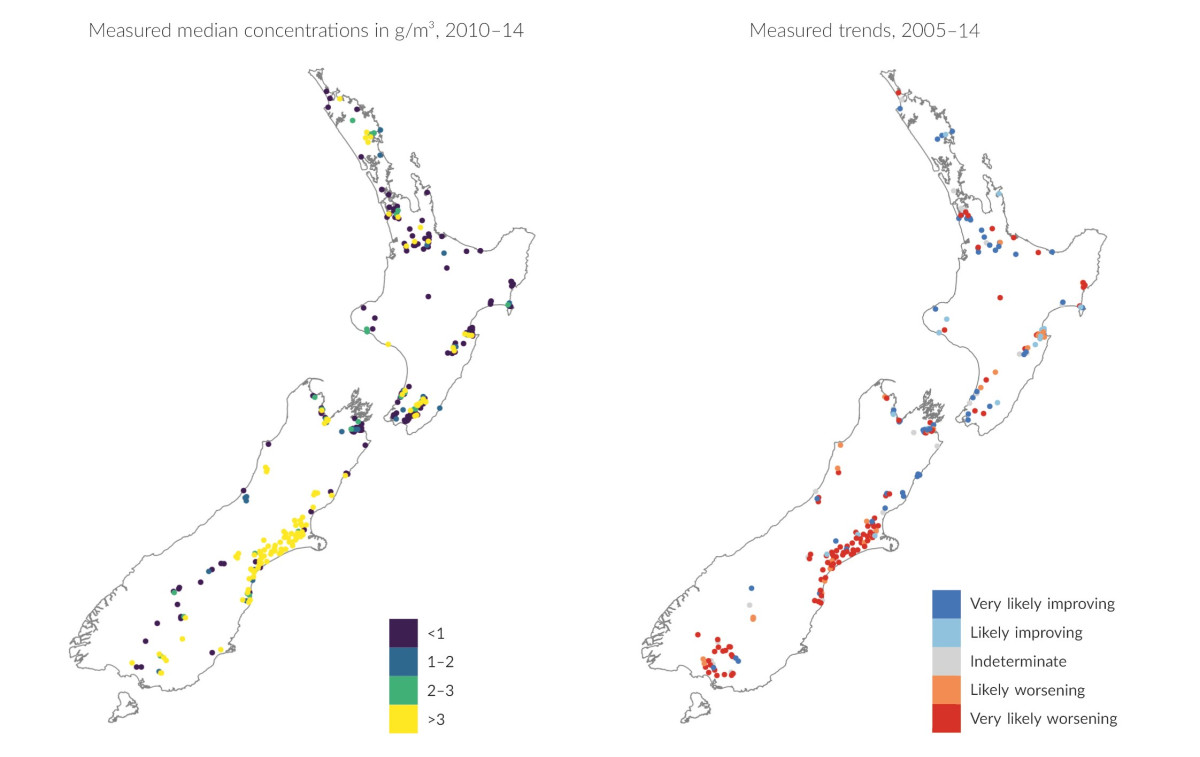
Image: Regional councils; GNS Science (Data source)
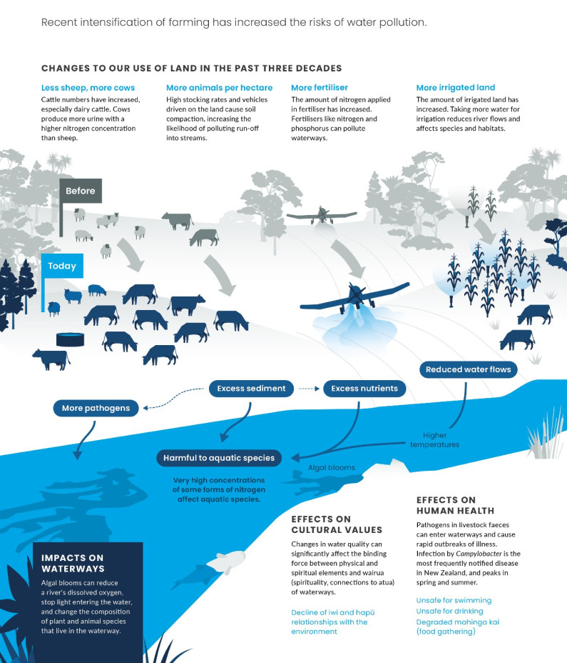

Read the long description for Intensified farming
Recent intensification of farming has increased the risks of water pollution
Changes to our use of land in the past three decades
Harmful to aquatic species
Impact on waterways
Effects on cultural values
Effects on human health
Changes in water quality are measured using trend tests. A worsening trend means that the amount of nitrogen, phosphorus, E. coli, or sediment is increasing over time so the water quality is likely to be worsening. An improving trend means that the concentration of these pollutants is decreasing.
More research is needed to understand how, where, and why trends in water quality occur, and why they speed up or slow down. The effects of natural climatic variations compared with the effects of human activities are also poorly understood (see Where are the gaps in our knowledge about this issue?).
In the 10 years from 2008 to 2017, some river water quality monitoring sites showed improving trends and some showed worsening trends. The pastoral and native land-cover classes had similar proportions of sites with improving and worsening trends (see figure 10). The absolute rate of change in both classes of land cover was less than 4 percent per year for most variables at most sites. (See indicators: River water quality: clarity and turbidity, River water quality: Escherichia coli, River water quality: macroinvertebrate community index, River water quality: nitrogen, and River water quality: phosphorus.)
Understanding the causes of these trends is difficult due to the complex interconnections between water bodies, variable lag times, and the mixture of land cover, land use, and land management that occurs in any given catchment (see What is the current state of this issue?).
The water quality in our rivers, groundwater, and lakes as reported above is generally similar to that in Our fresh water 2017, which reported on water quality using datasets ending between 2013 and 2015.
Trend assessments of water quality in this report, however, are based on improved methods (see Larned et al, 2018b; McBride, 2019; and Snelder & Fraser, 2018 for technical details).
The improved methods permit rates of change to be estimated more accurately at a larger number of sites. For example, this report uses data from at least 50 percent more river monitoring sites than were available for Our fresh water 2017.
The improved methods also allow trends to be classified according to their certainty:
By contrast, trends in Our fresh water 2017 used a 95 percent threshold to identify improving and worsening trends (as opposed to the 67 percent threshold used in this report). This means that Our fresh water 2017 reported a much higher proportion of sites as having indeterminate trends than this report.
The changes in trend assessment method and differences in available data mean that the trend results reported here are not directly comparable to those reported in Our fresh water 2017. These new methods for trend evaluation are, however, consistent with the approaches used by regional councils [Land, Air, Water Aotearoa website].

Image: NIWA (Data source)
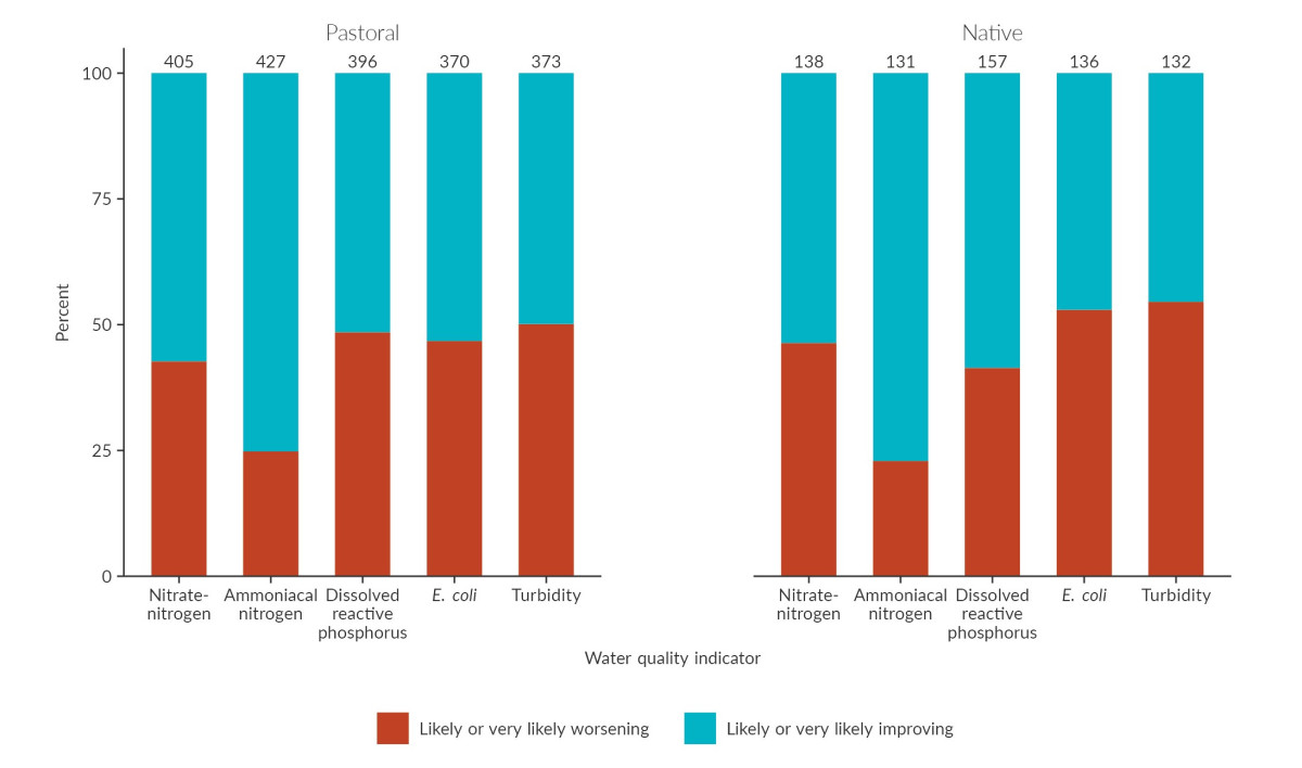
Image: NIWA (Data source)
Across all land-cover classes, the distribution of sites with improving versus worsening trends was not spatially uniform (see figure 11):
Lake, coastal, and estuarine water quality monitoring sites are not categorised by the amount of farmland in their catchments, so the impacts of farming cannot be specifically assessed.
Excluding sites with indeterminate trends, about two-thirds of groundwater sites had worsening trends in nitratenitrogen, ammoniacal nitrogen, and E. coli for 2005–14 (more recent national data had not been compiled at the time of writing this report). About half of the sites had worsening trends in dissolved reactive phosphorus in the same time period.
As with the assessment of the current state of groundwater quality, how farming has affected trends in groundwater quality cannot be assessed because monitoring sites are not categorised by land cover. However, some patterns coincide with pastoral land cover – especially for trends in nitrate-nitrogen in Canterbury (see figure 9 compared with figure 4).

Image: NIWA (Data source)
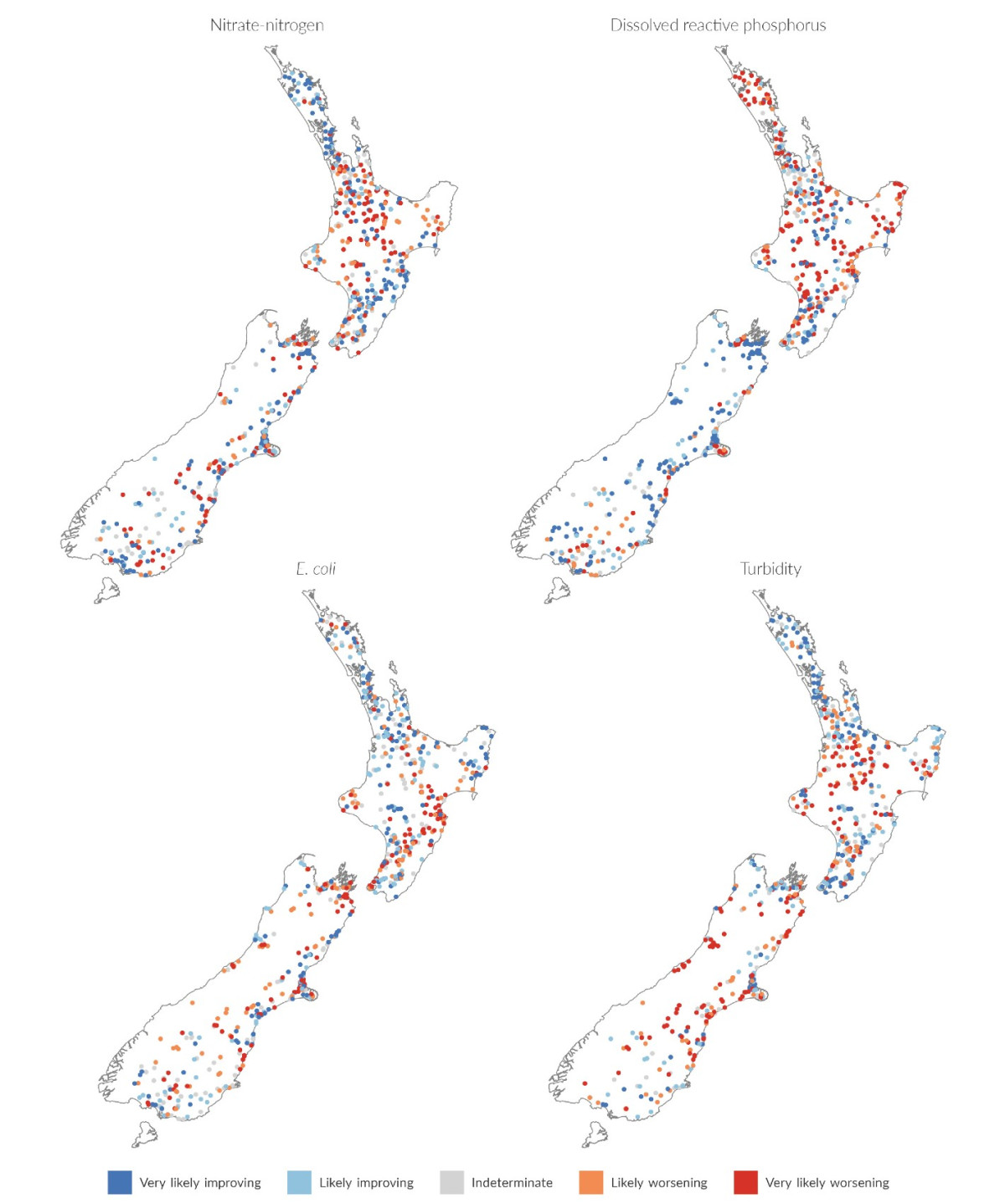
Image: NIWA (Data source)
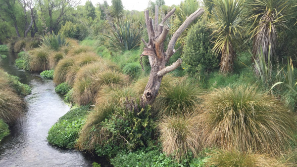
New native planting beside Ōtukaikino Creek. Photo credit: Arthur Adcock
Just south of the Waimakariri River in Christchurch is Ōtukaikino Creek. Fed by springs and groundwater, the small river is joined by water from a small wetland as it runs towards the east coast. This area was once used for burial preparations and is significant for Ngāi Tahu whānui.
The land was changed significantly by farming and urban development – native forest around the river was removed, the wetland became smaller, and the city grew. These changes combined to degrade the river’s water quality, with high levels of nutrients (nitrogen and phosphorus) and E. coli reported (LAWA, n.d.-a, n.d.-b). (See Issue 4: Our waterways are polluted in farming areas.)
Keeping farm animals away from rivers has many recognised benefits for the environment. It stops the animals causing direct damage to riverbanks by eroding the banks and adding sediment to the waterway, and trampling the places where birds live and make their nests. Fencing rivers also protects the riverside plants where native fish (like whitebait) lay their eggs (Richardson & Taylor, 2002). Dung and urine from the animals contain nutrients and pathogens (including E. coli) that reduce the water quality if they enter a waterway.
Following conversations between members of the community, landowners, and Arthur Adcock (a park ranger), a fencing and planting programme was begun in 2003. This was an essential part of its restoration. Farmers voluntarily fenced off 20–100-metre buffer zones between their stock and the river along almost its whole length, and an estimated 195,000 locally sourced native plants (including carex, flax, kahikatea, tōtara, and mātai) were planted in this area. Besides the cost of fencing, farmers also lost productive land and had to find new water sources for their animals.
Today, Ōtukaikino Creek has very good water quality. There have been substantial decreases in phosphorus levels in the past 10 years and concentrations of ammoniacal nitrogen, total nitrogen, and total oxidised nitrogen have also reduced. It is now a popular place for recreation, especially with a new walking track beside the river.
The wetland is now part of the 13-hectare Ōtukaikino Wildlife Management Reserve, which is being developed by the Department of Conservation with sponsorship from Lamb and Hayward. Long- and short-finned eel (tuna), flounder, whitebait, and native snails (pūpū) live there, as do pūkeko, shoveler (kuruwhengu), grey teal (tētē), and marsh crake (koitareke).
The collective actions of many people and organisations have contributed to the success of the restoration. Isaac Conservation and Wildlife Trust and Clearwater (a golf club and resort) helped create the large buffer zones that are thought to have made the restoration so successful. Department of Corrections community service workers weeded out species like willow and gorse and replanted with natives. Christchurch City Council, Fish and Game, Environment Canterbury, QEII National Trust, Department of Conservation, Trees for Canterbury, Z Energy (Aviation), local schools, Scout groups, and private landowners also made significant contributions.
Ōtukaikino Creek won the supreme award for most improved river at the New Zealand River Awards in 2018.
In less than 1,000 years New Zealand has changed from an unpopulated group of islands covered with dense forest, to an intensely farmed country dependent on export agriculture. Setting up our farms involved clearing native forests and scrub, and draining wetlands. These large-scale changes dramatically affected how our soils and water function. (See Issue 2: Changes to the vegetation on our land are degrading the soil and water.)
Establishing commercial agriculture also involved adapting imported farming systems to New Zealand conditions, including the use of fertiliser, trace elements, and irrigation to lift soil productivity. (See Issue 6: Taking water changes flows which affects our freshwater ecosystems.)
Several studies of river water quality indicate that an increasing proportion of agricultural land in an upstream catchment leads to increased concentrations of nitrogen, phosphorus, and E. coli, and sediment in waterways (Larned et al, 2018a).
While farming is not the only source for these pollutants, it is a major contributor:

Image: Stats NZ (Data source)
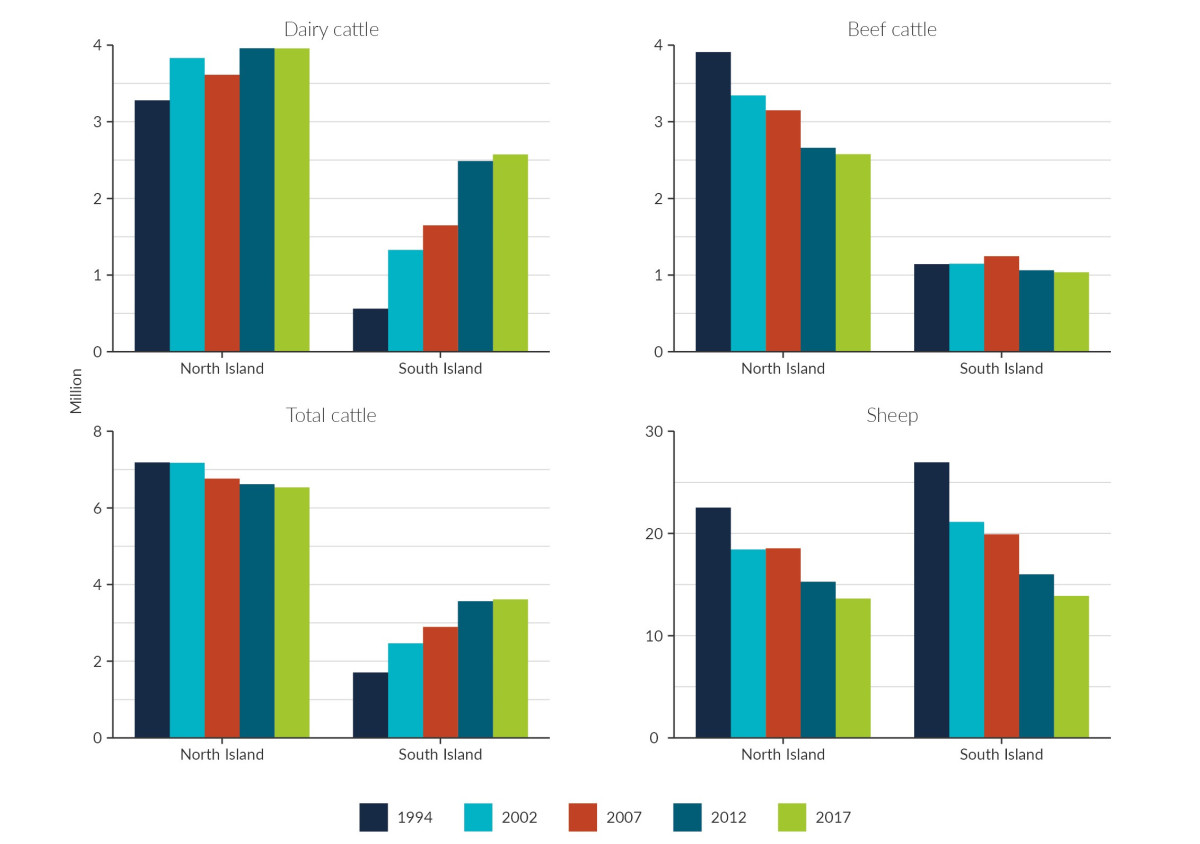
Image: Stats NZ (Data source)
From 1994 to 2017, the number of dairy cattle in New Zealand increased by 70 percent (from 3.8 million to 6.5 million). During the same period, the number of sheep decreased by 44 percent from 49.5 million to 27.5 million, and the number of beef cattle decreased by 28 percent from 5 million to 3.6 million. The increase in dairy cattle has been most pronounced in the South Island (see figure 12), notably in Canterbury, Otago, and Southland. (See indicator: Livestock numbers.)
The land area used for dairy farming has also increased. In 2016, the area of land used for dairy production was 2.6 million hectares (a 42 percent increase from 2002), while the area used for sheep and beef farming was 8.5 million hectares (a 20 percent drop in the same time). (See indicator: Agricultural and horticultural land use.)
This shift from sheep and beef farming to dairy farming is associated with increased leaching of nitrogen from agricultural soils. Cattle excrete more nitrogen per animal than sheep (cows produce more urine and the urine has a higher nitrogen concentration), so nitrogen from cattle is more likely to leach through soil than nitrogen from sheep (MfE, 2018).
When the concentration of nitrogen in animal dung and urine exceeds the amount that soil and plants can absorb, nitrogen is lost either through the soil into waterways, or into the air as a gas.
Models of the total amount of nitrate-nitrogen leached from livestock show this has increased from 189,000 tonnes per year nationwide in 1990 to about 200,000 tonnes per year in 2017. The amount of leaching in specific places has also changed as a result of shifts in the number and type of livestock around the country. According to the model, the highest nitrate-nitrogen leaching from livestock in 2017 occurred in Waikato, Manawatu-Wanganui, Taranaki, and Canterbury (see figure 13).
The modelling also shows that dairy cattle make a proportionally higher contribution to nitrogen leached from agricultural soils, compared with other types of livestock.
In 1990, 39 percent of modelled national nitrate-nitrogen leaching came from dairy cattle, 26 percent from beef cattle, and 34 percent from sheep. By 2017, nationally, dairy cattle contributed 65 percent of the modelled leached nitratenitrogen, with 19 percent from beef cattle and 15 percent from sheep. (See indicator: Nitrate leaching from livestock.)
A 2005 study estimated that nationally, 37 percent of the nitrogen load entering the sea came from dairy farming, despite dairying occurring on less than 7 percent of New Zealand’s land at that time (Elliot et al, 2005).
The number of cattle per hectare has increased between 1994 and 2017 in some areas of the country, notably Canterbury and Southland. (See indicator: Livestock numbers.)
More animals per paddock can contribute to nitrogen loss (Julian et al, 2017). When animals are closer together, there are more frequent and overlapping patches of urine, and a greater likelihood that soil and plant absorption will be overloaded (Ledgard, 2013).
High animal stocking rates and vehicles driven on the land can also cause soil compaction, particularly when the soil is wet (Drewry et al, 2008). Compaction closes up the small air spaces in the soil and reduces the drainage and leaching of nitrogen. The nitrogen on the surface of the soil can contribute to greenhouse gas emissions as nitrous oxide (N2O) more easily (van der Weerden et al, 2017) or be washed directly into waterways.
Use of nitrogen fertiliser has also increased. The amount of nitrogen applied in fertiliser has increased more than six-fold since 1990 – from 59,000 tonnes in 1990, to 429,000 tonnes in 2015. The amount of phosphorus applied as fertiliser annually peaked at 219,000 tonnes in 2005, but has reduced to about 150,000 tonnes per year in the last decade (155,000 tonnes in 2015). The risk of leaching depends on when the fertiliser is applied, eg in relation to rainfall, but data related to the timing of application is not available. (See indicator: Nitrogen and phosphorus in fertilisers.)
Some parts of the environment respond slowly to pressures. For example, it can take decades or more for groundwater (and the contaminants it contains) to move from the surface, through aquifers and back into surface water systems such as rivers, springs, lakes, or estuaries, and cause harm (Morgenstern & Daughney, 2012).
This creates a delay – known as lag time – between land-use impacts and their effects in a particular part of the environment. For example, in the catchment of Lake Rotorua, the average groundwater lag time is about 50 years and is more than 100 years in one catchment (Morgenstern et al, 2015).
As a result of long lag times, the water quality seen in some locations today may be the result of land use that occurred many years ago. It also means that, in some locations, today’s farming activities will not be seen to affect water quality for several years or even decades.

Image: Manaaki Whenua – Landcare Research (Data source)
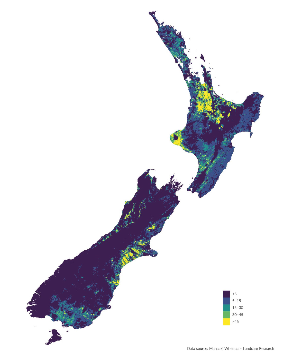
Image: Manaaki Whenua – Landcare Research (Data source)
Pollutants like nutrients and sediment begin to affect whole ecosystems as their concentrations increase. In extremely polluted waterways, very high concentrations of nitratenitrogen or ammonia are toxic to aquatic species.
One assessment of toxicity risk can be made by comparison of current water quality to the National Objectives Framework (NOF) bands for ecosystem health. NOF band A (the best water quality) describes conditions in which little or no toxicity risk is expected, even to the most sensitive aquatic species. In the native land-cover class, 98 percent of total river length is in NOF band A, based on the modelled concentrations of nitrate-nitrogen and ammonia. Only 29 percent of total river length in pasture-dominated catchments met this same condition.
NOF band D describes water quality that does not meet the national bottom line for a minimum acceptable state (ie where toxicity affects the growth and mortality of multiple sensitive species). None of New Zealand’s river lengths, in any land-cover class, had modelled concentrations of nitrate-nitrogen or ammonia in NOF band D. Likewise, the national bottom line for toxicity was not exceeded at any lake water quality monitoring sites.
Toxicity effects on groundwater ecosystems cannot be assessed because the effects of excess nutrients are not well known (Fenwick et al, 2018).
Algae, including cyanobacteria, occur naturally in rivers, lakes, and the sea (generally as periphyton – the natural growth on rocks and riverbeds – in shallow rivers, and as phytoplankton in deep rivers, lakes, and the sea). Algal blooms occur when the environmental conditions change and allow algae to reproduce rapidly. High concentrations of nitrogen and phosphorus, and warmer temperatures promote the growth and proliferation of these algae into a bloom.
National-scale information is not yet available to assess changes in periphyton biomass in rivers. Regional councils collect data on periphyton biomass (a requirement under the NOF) but this information does not yet provide a detailed national perspective. National-scale models have been developed to estimate periphyton biomass based on predictors such as nutrient concentrations, river flows, and the type of sediment on the riverbed, but these models have high uncertainty (Larned et al, 2015).
In lakes, the median TLI was rated poor or very poor at 57 percent of 58 monitored lake sites for 2013–17, indicating that frequent algal blooms were possible at these sites. The national bottom lines for total phosphorus, total nitrogen, and chlorophyll-a were not met at 17 percent, 30 percent, and 35 percent of the 63 monitored sites respectively during this period, indicating a high risk of degradation in lake ecological communities.
There is insufficient data to report on algal blooms or other indicators of eutrophication in coastal ecosystems.
An increasing frequency of algal blooms may have a range of consequences. Algal blooms can decrease the dissolved oxygen, prevent light from penetrating water, and change the composition of freshwater plant and animal species that live in a waterway. Some cyanobacteria produce toxins that can be harmful to ecosystems and contaminate water for drinking and swimming. Dogs are particularly susceptible because they are drawn to the odour of some cyanobacteria in rivers. More than 70 dog deaths have been reported across New Zealand since 2006 (Our fresh water 2017). Algal blooms may also degrade the recreational and cultural uses of waterways.
The presence of E. coli bacteria above a certain limit is used to assess the health risk from the pathogen Campylobacter in rivers and lakes. Infection by Campylobacter can cause gastrointestinal illness and is the most frequently notified disease in New Zealand, peaking in spring and summer (Ministry of Health, 2018).
Computer models (Whitehead, 2018) can be used to estimate the average Campylobacter infection risk from swimming in any New Zealand river. For 2013–17, 82 percent of the river length in the pastoral land-cover class was not suitable for activities such as swimming, based on a predicted average Campylobacter infection risk of greater than 3 percent (NOF bands D and E respectively – the two highest risk categories). Only 5 percent of the river length in the native land-cover class exceeded the same threshold.
Regional councils monitor popular swimming sites, including rivers, lakes, and coastal areas, to assess the health risk. For the most up-to-date information on your local swimming spot, see the Land, Air, Water Aotearoa website.
Monitoring untreated water in aquifers for 2010–14 found that 59 percent of 147 sites failed to meet the drinking water standard for E. coli on at least one occasion. (This indicates a potential risk of illness if the water is ingested without being treated.) The drinking water standard of 11.3 grams per cubic metre of nitrate-nitrogen was exceeded on at least one occasion at 13 percent of 364 sites tested. (At this concentration, nitrate-nitrogen has a potential risk of causing methaemoglobinaemia, blue baby syndrome, in bottle-fed infants.)
This monitoring contributes to a picture of the overall quality of our groundwater. Information is not available about which of these monitoring wells are actually used for drinking water, which wells are situated in farming areas, and whether treatment is in place to remove pathogens and nitrate-nitrogen from well water.
A large proportion of New Zealand’s drinking water comes from rivers and underground aquifers and is tested and treated to make it safe to drink.
The concentration of pesticides in surface waters is not routinely measured, but groundwater monitoring shows that pesticides in the water in aquifers currently pose a low risk to health (Our fresh water 2017).
Changes in water quality can significantly affect the mauri (binding force between physical and spiritual elements) (Morgan, 2006) and wairua (spirituality, connections to atua) of waterways. Degraded waterways can affect the perception of mana (prestige) associated with an iwi or hapū (Our fresh water 2017). The health and capacity of our waterways to provide is a significant part of expressing ahikāroa (connection with place) and kaitiakitanga (guardianship).
Customary practices associated with mahinga kai (food gathering area) from waterways contribute significantly to manaakitanga (acts of giving and caring for), whanaungatanga (community relationships and networks), te ahurea o te reo (growth and evolution of language), and whakaheke kōrero (opportunities for inter-generational transfer of mātauranga) (Harmsworth & Awatere, 2013; Lyver et al, 2017a; Royal, 2007; Timoti et al, 2017).
Some iwi and hapū monitor fresh water using cultural indicators (like the time it takes to collect enough pipi for a family meal) to record changes in the health of these areas. Our fresh water 2017 reported on a cultural health index (CHI) for water quality (see indicator: Cultural health index for freshwater bodies) made up of three elements:
Of 41 sites at which CHI was assessed between 2005 and 2016, 11 sites had very good or good scores, 21 sites had moderate scores, and 9 sites had poor or very poor scores. Sites were not classified according to land cover so the impacts of farming cannot be specifically assessed.
Data clearly shows that at a national scale, water quality in pastoral farming areas is degraded. Horticulture and arable cropping can also affect water quality (Larned et al, 2018a), though these cover much less area than pastoral farming. At a local scale, however, there is insufficient information and knowledge about exactly where, when, and what specific activities and management practices (eg tillage, effluent management) have contributed to (or mitigated) water pollution in farming areas (Larned et al, 2018a; McDowell et al, 2019).
This is partly because there is no national-scale database or map of farm management practices. Furthermore, in locations with long lag times (see Lag times can be long), the current water quality may be the result of past management practices, rather than what we are doing now. More information is therefore needed about the flow of pollutants as they move through catchments – including the locations, sizes, and properties of New Zealand’s aquifers, and where and how groundwater and surface waters interact.
There is also poor understanding of the causes of water quality trends. Some trends may be caused by variations in climate or other natural processes that are currently not accounted for, so the contribution of human activities is difficult to determine. At some locations it may be challenging to distinguish input of nutrients from farming from other sources like wastewater treatment systems.
Because of these large knowledge gaps, it is hard to assess the impacts on water quality from specific land management practices like stocking density, fertiliser use, and the disposal of agricultural effluent, or measure improvements in water quality arising from specific actions like riparian planting.
There is a lack of knowledge about how changes in water quality affect the health of an ecosystem. A framework to describe ecosystem health holistically has been developed (Clapcott et al, 2018), but work is still underway to choose the parameters to evaluate it. (See Issue 1: Our native plants, animals, and ecosystems are under threat.) National datasets for some variables relevant to ecosystem health is still lacking (like deposited sediment, continuous dissolved oxygen, and algal biomass). There is also insufficient information about biodiversity and native fish populations, including taonga species (Our fresh water 2017). Very little is known about groundwater ecosystems. Also, the interacting and cumulative effects of water pollution and other pressures on ecosystem health are not well understood (Larned et al, 2018a).
There is a critical gap in our knowledge about the impacts of water pollution on te ao Māori, particularly how mātauranga Māori, tikanga Māori, kaitiakitanga, customary use, and mahinga kai are affected. Although some relevant datasets are available (like information about traditional freshwater crayfish (kōura) gathering), we lack information about how changes in land use affect Māori values for fresh water (Larned et al, 2018a).
Information about the impacts of water pollution on human health is also poor. Regional authorities carry out water quality monitoring at approximately 150 of New Zealand’s lakes and E. coli is monitored at very few of these (Larned et al, 2019). New research programmes are just beginning to collect data on emerging contaminants in our waterways. These include pesticides, pharmaceuticals, nanoparticles, and other chemicals that are now found more commonly in waterways overseas (Petrie et al, 2015).
Some of our cities and towns have polluted air, land, and water. This comes from home heating, vehicle use, industry, and disposal of waste, wastewater, and stormwater. Pollution affects ecosystems, health, and use of nature.
It can apply to all cities and towns.
The type and severity of pollution varies from place to place and over time.
It is challenging to reverse because changing our cities and lifestyles would require significant investment and changes in behaviour.
There is high risk to human health and cultural well-being, practices, and knowledge because 86 percent of New Zealanders live in an urban centre. Fresh water, marine, air, and atmosphere can all be affected.
Data for all pollutants in urban areas is lacking. Their cumulative impacts on human health, ecosystems, and cultural well-being are not known.
Many different pollutants are produced in urban centres, from home heating, vehicle use, industry, waste disposal, wastewater, and stormwater. The pollutants vary in type and amount from place to place and over time. Although some pollutants occur naturally, in urban areas pollution comes mostly from human activities and can accumulate to harmful levels in air, land, freshwater, and marine environments.
In the most recent national land-cover assessment (2012), urban areas covered 0.8 percent of our land. (See indicator: Urban land cover.) Our urban centres have been growing – urban land area increased by 10 percent between 1996 and 2012. (See Issue 3: Urban growth is reducing versatile land and native biodiversity.)
About 86 percent of New Zealanders lived in an urban centre in 2013 – 73 percent in a city or a major urban area (more than 30,000 people), 6 percent in a large regional centre (10,000–29,999 people), and 8 percent in smaller towns (1,000–9,999 people) (Stats NZ, n.d.-a).
There is also some evidence of increasing population density. From 1996–2013 the density of Auckland’s urban area rose from 21 people per hectare to 25 people per hectare (Auckland Council, 2014).
Our air quality is good in most places and at most times of the year, particularly when compared with heavily industrialised countries (Our air 2018). The most common air pollutants in urban areas are gases like nitrogen dioxide (NO2), sulphur dioxide (SO2), ozone (O3), and carbon monoxide (CO), and very fine particles or particulate matter (PM). Particulate matter is often classified by its size. PM10 has a diameter of 10 micrometres (μm) or less. PM2.5 has a diameter of less than 2.5 μm and is therefore a subset of PM10. Generally, the smaller the particles, the greater the risk to human health.
PM levels can exceed standards and guidelines, especially in cooler months due to emissions from home heating, and when calm weather and the landscape allow pollutants to build up in the air (see figure 14).
Less data is available for gaseous air pollutants. The available measurements show that SO2 levels can exceed environmental standards at some locations, whereas exceedances of NO2 standards are less common. The concentrations of O3 and CO are low and are unlikely to exceed the standards (Our air 2018). (See indicators: Nitrogen dioxide concentrations, Sulphur dioxide concentrations, Ground-level ozone concentrations, and Carbon monoxide concentrations.)
Light pollution, noise pollution, and odours can also be polluting (Our air 2018). Light pollution is very low in most parts of New Zealand but all our large urban areas have levels of artificial light that can affect visibility of the night sky. (See indicator: Artificial night sky brightness.) Data for noise pollution and odours is not available for New Zealand.

Image: Regional councils and unitary authorities (Data source)
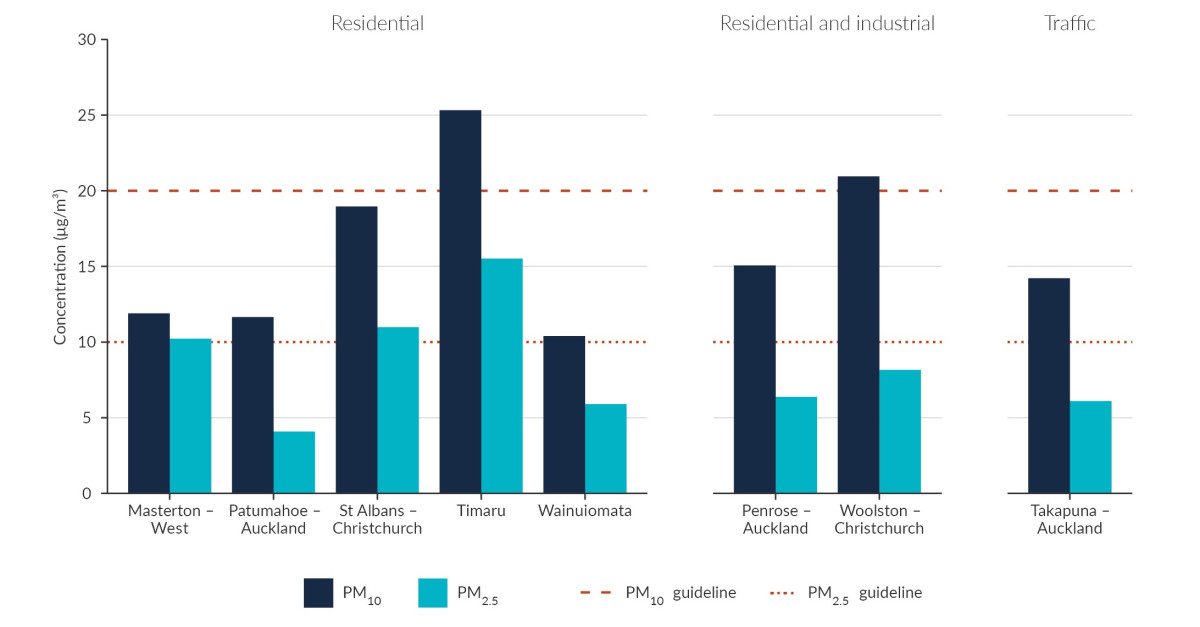
Image: Regional councils and unitary authorities (Data source)
Computer models are used to estimate the median concentrations of nutrients, Escherichia coli (E. coli), clarity, and turbidity in New Zealand waterways for 2013–17 (Whitehead, 2018). (See Issue 4: Our waterways are polluted in farming areas and indicators: River water quality: clarity and turbidity, River water quality: Escherichia coli, River water quality: nitrogen, and River water quality: phosphorus.)
The models show that, for most water quality variables, over 80 percent of the total river length in the urban land-cover class exceeds the relevant default guideline value (DGV) (see table 2). In comparison, the models show that DGVs are exceeded by slightly lower percentages of river length in the pastoral land-cover class and less than 30 percent of the river length in the native land-cover class (compare with table 1). (In total, 3,344 kilometres of New Zealand’s river length is in the urban land-cover class, compared with 188,024 kilometres in the pastoral landcover class, and 198,126 kilometres in the native landcover class.)
These models also show that river water quality in urban areas was much worse than expected for natural conditions for 2013–17 (see table 2). For these stretches (or reaches) of urban rivers, modelled median nitrate-nitrogen levels were 19.5 times higher, dissolved reactive phosphorus levels 4.7 times higher, turbidity 3.3 times higher, and E. coli 30 times higher than in river reaches dominated by native land cover. The river water quality in urban areas was even poorer than in pastoral areas for the same time period, based on the modelled median concentrations of these pollutants (compare with table 1).
Heavy metals also commonly pollute urban streams – the concentration of copper and zinc increases with the proportion of urban land in the catchment. Monitoring data for 2013–15 show that dissolved zinc and copper concentrations in urban streams in Auckland, Wellington, and Christchurch are higher than in non-urban areas. (See indicator: River water quality: heavy metals.)
Wastewater and stormwater can also contain pollutants such as pesticides, pharmaceuticals, personal care products, and other substances that are not adequately removed by treatment plants (Petrie et al, 2015). Many types of litter (including plastic) can end up on land, be washed into waterways, and may eventually reach the ocean. Data for these emerging pollutants in New Zealand waterways is not available.
Groundwater and lake water quality monitoring sites are not categorised according to land use, so the specific effects of urban land cover on these water bodies cannot be identified.
| Modelled median value of water quality variable, 2013–17 | River length (km) that does not meet ANZG DGV | ||||
|---|---|---|---|---|---|
| Water quality variable | Units | Urban land cover | Native land cover | Urban land cover | Native land cover |
| Total nitrogen | mg/m3 | 992.2 | 115.9 | 3,153 (94%) | 57,027 (29%) |
| Nitrate-nitrogen | mg/m3 | 497.8 | 25.6 | 3,214 (96%) | 26,610 (13%) |
| Ammoniacal nitrogen | mg/m3 | 29.9 | 4.0 | 3,020 (90%) | 29,464 (15%) |
| Total phosphorus | mg/m3 | 43.3 | 8.3 | 3,267 (98%) | 50,977 (26%) |
| Dissolved reactive phosphorus | mg/m3 | 20.5 | 4.4 | 3,104 (93%) | 45,270 (23%) |
| E. coli | cfu/100ml | 399.9 | 13.3 | 1,512 (45%) | 1,117 (0.6%) |
| Turbidity | NTU | 4.4 | 1.3 | 2,276 (68%) | 22,962 (12%) |
| Clarity | m | 1.5 | 3.3 | 163 (5%) | 1,467 (1%) |
Note: ANZG (2018) does not include a DGV for E. coli, so the expected concentration for natural conditions is based on the guideline value determined by McDowell et al (2013). Because of the way a DGV is defined, even under natural conditions, it is expected that about 20 percent of river length will not meet the DGVs and about 5 percent of river length will not meet the E. coli guideline.
Coastal water quality is strongly affected by the polluting nutrients, pathogens, and sediment that are carried downstream by rivers (Dudley et al, 2017). (See Issue 4: Our waterways are polluted in farming areas.) Monitoring data for 2013–17 showed that high nitrogen concentrations and high levels of faecal bacteria occurred at the coastal sites with high river inflows, particularly in tidal estuaries with short residence times. Deep estuaries had the best water quality because they tended to receive less contamination from rivers. (See indicator: Coastal and estuarine water quality.)
The land cover upstream from coastal monitoring sites has not been categorised, so the proportion of nutrients, pathogens, and sediment delivered from urban areas, as opposed to other land uses such as farming, is not known.
Heavy metals are known to reach estuaries primarily via urban streams (with the exception of cadmium, which can also come from farming areas). Data at most monitoring sites in 13 regions for 2015–2018, however, showed that the concentration of heavy metals in estuarine and coastal sediment was below the levels expected to affect benthic species. (See indicator: Heavy metal load in coastal and estuarine sediment.)
Industrial, commercial, and domestic activities can all contaminate soil in urban areas. Historic activities can continue to contaminate soil for decades.
Although the types of contamination that occur in New Zealand are known, there is not enough data to report on their extent or magnitude here (Our land 2018).
PM10 concentrations decreased in 17 of 39 monitored areas (airsheds) in winter between 2007 and 2016. This data is from 47 monitoring sites that are mostly in residential areas. (See indicators: PM10 concentrations and PM2.5 concentrations.) NO2 concentrations improved at 23 sites and worsened at 3 sites for 2010–16, as recorded at 92 urban monitoring sites across the country. Few monitoring sites have sufficient data to assess trends in SO2, O3, or CO. No data is available to assess trends in light pollution, noise pollution, or odours.
Excluding sites with indeterminate trends, about 75 percent of urban river water monitoring sites for 2008–17 had improving trends for nitrate-nitrogen, ammoniacal nitrogen, dissolved reactive phosphorus, and turbidity. Approximately half of the sites had improving trends for E. coli (see figure 15).
More urban river sites had improving trends for nitrate-nitrogen, dissolved reactive phosphorus, and turbidity than sites with pastoral or native land cover during this time. Monitored sites with urban, pastoral, and native land cover had similar proportions of improving and worsening trends for ammoniacal nitrogen and E. coli.
The absolute rate of change at sites in the urban land-cover class was less than 4 percent per year for most variables at most sites for 2008–17. (See Issue 3: Urban growth is reducing versatile land and native biodiversity.)
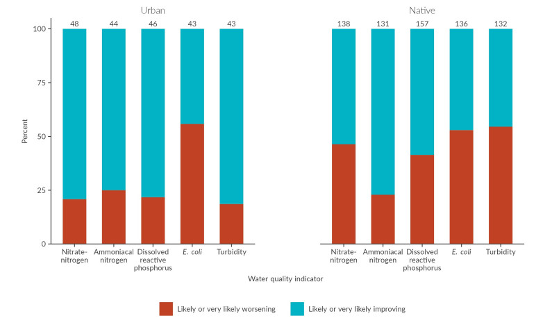
Image: NIWA

Image: NIWA
In coastal environments, for most water quality variables, more sites show improving trends than worsening trends for 2008–17. Levels of Enterococci (used instead of E. coli as an indicator in coastal waters) were decreasing at 41 percent of monitored sites. Only total nitrogen, ammoniacal nitrogen, and dissolved oxygen showed a greater proportion of sites with worsening trends in this period. However, the monitoring sites were not categorised according to the land cover upstream so the effects of urban areas, as opposed to other land uses such as farming, cannot be assessed. There is not enough data to assess trends in the concentrations of heavy metals in coastal and estuarine sediments.
Regional councils keep records of sites where land contamination has been confirmed, but there is currently no integrated dataset available for the national scale. A number of previously unreported contaminants have been found recently in some areas (Our land 2018). These include per-and poly-fluoroalkyl substances (PFAS). These chemicals have many uses including waterproofing and printing, and were used historically in foams for fighting flammable liquid fires at airfields and fuel storage facilities.
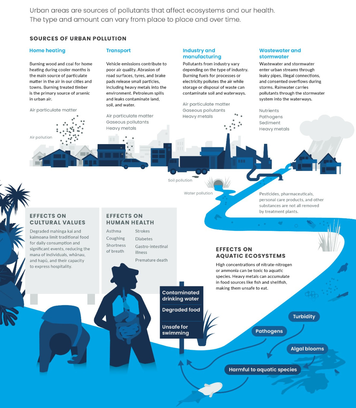
The most common human-made source of PM in our urban atmospheres is emissions from burning fuels like wood and petrol. Home heating emissions (burning wood and coal) produced 25 percent of PM10 and 33 percent of PM2.5 in 2015, mainly in urban areas. (See indicator: Air pollutant emissions.) Burning treated timber to heat homes is also the primary source of arsenic in urban air (Cavanagh et al, 2012).
Vehicle emissions contribute to poor air quality in some places. Cars typically emit air pollutants including PM, carbon dioxide (CO2), CO, volatile organic compounds (VOCs, as unburned hydrocarbons), and oxides of nitrogen (NOx). Wear and abrasion of road surfaces, tyres, and brake pads also release small particles that can be a significant source of heavy metals like zinc, cadmium, barium, antimony, and copper (Schauer et al, 2006).
Spills and leaks of petroleum fuels at storage facilities, including service stations, can contaminate land, soil, and water (Our land 2018).
Ships are another important source of air pollutants in coastal urban areas (mainly SO2 but also NO2 and PM) because many ports are located close to city centres.
Burning fuel to power industrial processes or generate electricity (in wood- or coal-fired boilers for example) can produce air pollution. Pollutants can also be emitted from the processes themselves, like the gases released during smelting. Pollutants emitted by industry are as varied as the industries that produce them and can include NOx, SO2, CO2, VOCs, PM, and heavy metals (Our air 2018). Industrial pollutants can end up in urban soil, waterways, and on land.
Although there is no database of confirmed contaminated land in New Zealand, the Resource Management Act survey of local authorities 2012/2013 (MfE, 2014) reported 19,568 sites nationwide where activities and industries are considered likely to cause land contamination from the use, storage, or disposal of hazardous substances. Not all of these sites are in urban areas.
In urban environments, pollutants enter waterways through the stormwater and wastewater networks. (Stormwater is rainwater plus any pollutants it picks up on the land surface, while wastewater is the water used in houses, businesses, and industrial processes.) Pollutants can enter urban streams through illegal connections to wastewater and stormwater networks, and leaky pipes, and pumps. Pollutants from urban streams can be carried into rivers, aquifers, estuaries, and coastal areas.
Nutrients and faecal pathogens are common pollutants in wastewater. Nutrients can also enter the stormwater system from spills or fertiliser used on lawns and golf courses (Our fresh water 2017). Stormwater can contain elevated concentrations of heavy metals (Lewis et al, 2015), coming from vehicles (copper from brake pads and zinc from tyres), metal roofing, and industrial yards (Kennedy & Sutherland, 2008). Wastewater and stormwater can also contain many other pollutants including personal care products, medicines, and plastics that were washed into waterways.
The extent to which stormwater and wastewater pollute fresh water is determined by how much land is covered by solid surfaces like roofing, asphalt, and concrete. These impervious surfaces reduce the amount of rain that soaks into soils and aquifers, and increase the amount entering the stormwater system.
The design, maintenance, and operation of infrastructure also affect water pollution in urban areas. Many stormwater and wastewater networks have consented overflows for storms, so during these times, wastewater can flow into stormwater systems (Our fresh water 2017). Better wastewater treatment may be associated with the improvement in water quality reported in urban streams (Davies-Colley, 2013). However, nationally, one-quarter of wastewater assets are more than 50 years old, with 10–20 percent of the network requiring significant renewal or replacement (LGNZ, 2014).

Read the long description for Urban pollution
Urban areas are sources of pollutants that affect ecosystems and our health. The type and amount can vary from place to place and over time.
Sources of urban pollution
Pesticides, pharmaceuticals, personal care products, and other substances are not all removed by treatment plants.
Effects on cultural values
Effects on human health
Effects on aquatic ecosystems
Algal blooms and the growth of cyanobacteria (see Issue 4: Our waterways are polluted in farming areas) are more likely in waterways with higher concentrations of nutrients. The concentrations of nitrogen and phosphorus are much higher in rivers in urban areas than those with native vegetation, so the likelihood of blooms is higher in these environments (if other necessary conditions for algal growth are met).
Very high concentrations of nitrate-nitrogen or ammonia can be toxic to aquatic species. Whereas 98 percent of river length in the native land-cover class had modelled median concentrations of nitrate-nitrogen and ammonia that were expected to pose little or no toxicity risk to aquatic species, only 6 percent of river length in the urban land-cover class met this same condition (as did 29 percent of river length in the pastoral land-cover class).
High concentrations of heavy metals can also be toxic to aquatic species. For 2013–15, the concentrations of dissolved copper and dissolved zinc exceeded toxicity guidelines for 12 of 17, and 27 of 50 urban sites, respectively (Gadd, 2016). The current levels of heavy metals in estuary sediments are mostly unlikely to cause harm to seabed species.
Air pollution can cause coughing, shortness of breath, heart attack, stroke, diabetes, and premature death (Our air 2018). Studies that are specific to New Zealand are limited, but models estimate that there were 27 premature deaths per 100,000 people from exposure to PM10 in 2016. Per capita, the number of premature deaths was estimated to be 8 percent lower in 2016 than in 2006, mostly because more people were living in areas with lower PM10, like Auckland, rather than a reduction in overall PM10 (Our air 2018). (See indicator: Health impacts of PM10.)
Pollution of urban waterways and coasts by faecal pathogens can make water unsafe for swimming. Regional councils monitor popular swimming sites, including rivers, lakes, and coastal areas to assess the level of health risk for recreational activities (see Land, Air, Water Aotearoa website).
Nationwide estimates of the average Campylobacter infection risk from river water are made by modelling the median E. coli concentration (Whitehead, 2018). For 2013–17, 94 percent of the total river length in the urban land-cover class was not suitable for activities such as swimming, based on a predicted average Campylobacter infection risk of greater than 3 percent (National Objectives Framework (NOF) bands D and E, which are the two highest risk categories). For the pastoral land-cover class, the same Campylobacter infection risk was estimated at 82 percent of river length but only 5 percent in catchments in the native land-cover class.
Heavy metals can accumulate in food sources like fish and shellfish, making them unsafe to eat. Data from monitored sites indicate that this is a low risk.
Pollution in urban areas impacts the mauri of ecosystems and affects values like the condition of mahinga kai and kaimoana (traditional foods), recreation (swimming, waka ama), and oranga (health and well-being) of Māori (Harmsworth & Awatere, 2013; Madarasz-Smith, 2013). It also significantly diminishes the existence and capacity of waterways and ecosystems to sustain and provide for the spiritual, cultural, and physical needs of hapū and whānau.
The effects can be critical, for example, the inability of hapū and whānau to access and maintain mahinga kai and kaimoana, in turn, impacts the mana of those groups by limiting their ability to sustain themselves and express manaakitanga (hospitality, generosity). In addition, the loss of access to native species (through biodiversity degradation) over time constrains the ability to express kaitiakitanga and to maintain the knowledge and practice that accompanies that responsibility.
The responsibility of kaitiakitanga extends to air and light quality (Kuschel et al, 2012; Scheele et al, 2016), so pollution could negatively affect cultural practices including reading tohu (signs or indicators, eg during Matariki), navigation, and using maramataka (Māori lunar calendar).
Many of the knowledge gaps identified in Issue 4: Our waterways are polluted in farming areas also apply to urban pollution.
There is clear evidence that levels of pollutants like nutrients, pathogens, sediment, and heavy metals in waterways, and air particulate matter are higher in urban than non-urban areas, but the sources of urban pollution can be very localised and vary significantly over short time periods. Monitoring networks do not yet cover all our cities and towns and are notably lacking for land and soil. Time-series datasets that are long enough and have high enough resolution are not available for some pollutants. There is also no data to evaluate new issues like indoor air quality or emerging contaminants in fresh water and land.
There is limited understanding of how urban pollution affects the things we value. Data to measure the impacts of pollution on ecosystems and cultural values is lacking. A particular challenge arises when or where many different types of pollutants are present simultaneously because of their combined and interacting effects. Such cumulative effects may also be compounded by other pressures acting on the environment, like habitat modification, introduced pests, and modified water flows.

Theme 3: Pollution from our activities
April 2019
© Ministry for the Environment